Store Color and Coordinates in a Table Pixel Art Javascript

• Home
• Guides
• Reference
• Support
• Community
• Deject
• Information Itemize

Image Visualization

The are a number of ee.Image methods that produce RGB visual representations of prototype data, for example: visualize(), getThumbURL(), getMap(), getMapId() (used in Colab Folium map display) and, Map.addLayer() (used in Lawmaking Editor map display, not available for Python). By default these methods assign the outset 3 bands to carmine, green and blue, respectively. The default stretch is based on the type of data in the bands (e.g. floats are stretched in [0, one], 16-scrap data are stretched to the full range of possible values), which may or may not exist suitable. To reach desired visualization furnishings, y'all can provide visualization parameters:

Image visualization parameters

Parameter	Description	Type
bands	Comma-delimited listing of three band names to exist mapped to RGB	list
min	Value(south) to map to 0	number or list of iii numbers, ane for each band
max	Value(s) to map to 255	number or listing of iii numbers, one for each ring
gain	Value(s) by which to multiply each pixel value	number or list of three numbers, ane for each band
bias	Value(southward) to add to each DN	number or list of three numbers, one for each ring
gamma	Gamma correction factor(s)	number or listing of iii numbers, one for each ring
palette	List of CSS-fashion color strings (single-band images only)	comma-separated list of hex strings
opacity	The opacity of the layer (0.0 is fully transparent and 1.0 is fully opaque)	number
format	Either "jpg" or "png"	string

RGB composites

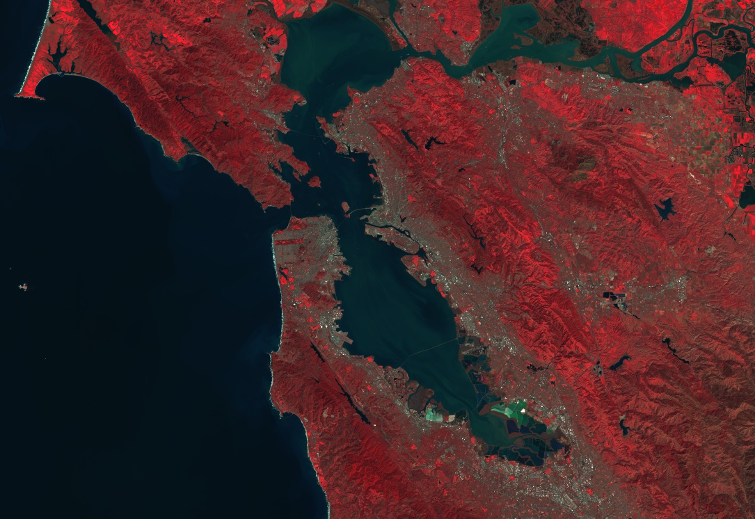
The following illustrates the use of parameters to style a Landsat eight image as a false-color blended:

Lawmaking Editor (JavaScript)

// Load an prototype. var epitome = ee.Image('LANDSAT/LC08/C02/T1_TOA/LC08_044034_20140318');  // Define the visualization parameters. var vizParams = {   bands: ['B5', 'B4', 'B3'],   min: 0,   max: 0.5,   gamma: [0.95, ane.i, 1] };  // Center the map and display the image. Map.setCenter(-122.1899, 37.5010, 10); // San Francisco Bay Map.addLayer(image, vizParams, 'false color composite');

Colab (Python)

# Load an image. image = ee.Image('LANDSAT/LC08/C02/T1_TOA/LC08_044034_20140318')  # Define the visualization parameters. image_viz_params = {     'bands': ['B5', 'B4', 'B3'],     'min': 0,     'max': 0.v,     'gamma': [0.95, 1.one, 1] }  # Define a map centered on San Francisco Bay. map_l8 = folium.Map(location=[37.5010, -122.1899], zoom_start=ten)  # Add the image layer to the map and display it. map_l8.add_ee_layer(image, image_viz_params, 'fake colour blended') brandish(map_l8)

In this example, band 'B5' is assigned to cherry-red, 'B4' is assigned to green, and 'B3' is assigned to blue.

Landsat 8 simulated color composite of San Francisco bay area, California, USA.

Color palettes

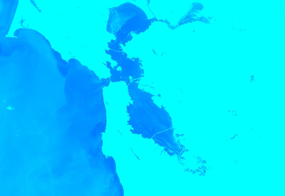
To display a single band of an image in color, set the palette parameter with a color ramp represented by a list of CSS-way color strings. (Run across this reference for more information). The post-obit instance illustrates how to use colors from cyan ('00FFFF') to blue ('0000FF') to render a Normalized Difference H2o Index (NDWI) epitome:

Lawmaking Editor (JavaScript)

// Load an image. var image = ee.Image('LANDSAT/LC08/C02/T1_TOA/LC08_044034_20140318');  // Create an NDWI image, define visualization parameters and display. var ndwi = paradigm.normalizedDifference(['B3', 'B5']); var ndwiViz = {min: 0.5, max: 1, palette: ['00FFFF', '0000FF']}; Map.addLayer(ndwi, ndwiViz, 'NDWI', false);

Colab (Python)

# Load an image. image = ee.Image('LANDSAT/LC08/C02/T1_TOA/LC08_044034_20140318')  # Create an NDWI epitome, define visualization parameters and display. ndwi = prototype.normalizedDifference(['B3', 'B5']) ndwi_viz = {'min': 0.v, 'max': one, 'palette': ['00FFFF', '0000FF']}  # Define a map centered on San Francisco Bay. map_ndwi = folium.Map(location=[37.5010, -122.1899], zoom_start=10)  # Add the image layer to the map and display it. map_ndwi.add_ee_layer(ndwi, ndwi_viz, 'NDWI') display(map_ndwi)

In this example, note that the min and max parameters indicate the range of pixel values to which the palette should be applied. Intermediate values are linearly stretched.

Too note that the show parameter is set to simulated in the Lawmaking Editor example. This results in the visibility of the layer being off when it is added to the map. It can always be turned on again using the Layer Manager in the upper right corner of the Lawmaking Editor map.

Landsat 8 NDWI, San Francisco bay area, The states. Cyan are low values, blueish are high values.

Masking

You can utilize image.updateMask() to set the opacity of individual pixels based on where pixels in a mask image are non-zero. Pixels equal to zero in the mask are excluded from computations and the opacity is prepare to 0 for display. The following instance uses an NDWI threshold (see the Relational Operations department for information on thresholds) to update the mask on the NDWI layer created previously:

Code Editor (JavaScript)

// Mask the non-watery parts of the image, where NDWI < 0.iv. var ndwiMasked = ndwi.updateMask(ndwi.gte(0.four)); Map.addLayer(ndwiMasked, ndwiViz, 'NDWI masked');

Colab (Python)

# Mask the not-watery parts of the image, where NDWI < 0.iv. ndwi_masked = ndwi.updateMask(ndwi.gte(0.four))  # Define a map centered on San Francisco Bay. map_ndwi_masked = folium.Map(location=[37.5010, -122.1899], zoom_start=10)  # Add the image layer to the map and brandish it. map_ndwi_masked.add_ee_layer(ndwi_masked, ndwi_viz, 'NDWI masked') display(map_ndwi_masked)

Visualization images

Employ the epitome.visualize() method to convert an image into an 8-bit RGB image for display or export. For example, to catechumen the false-color composite and NDWI to 3-band display images, utilize:

Code Editor (JavaScript)

// Create visualization layers. var imageRGB = paradigm.visualize({bands: ['B5', 'B4', 'B3'], max: 0.five}); var ndwiRGB = ndwiMasked.visualize({   min: 0.5,   max: one,   palette: ['00FFFF', '0000FF'] });

Colab (Python)

image_rgb = epitome.visualize(**{'bands': ['B5', 'B4', 'B3'], 'max': 0.5}) ndwi_rgb = ndwi_masked.visualize(**{     'min': 0.5,     'max': 1,     'palette': ['00FFFF', '0000FF'] })

Mosaicking

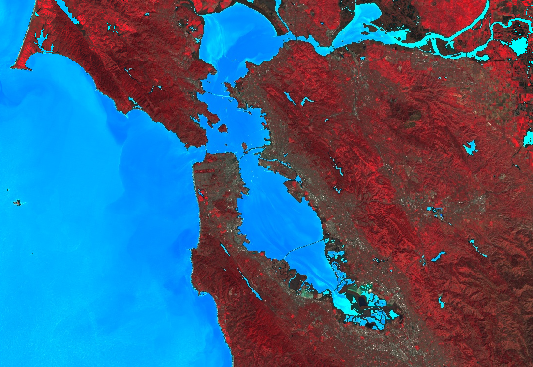
You can apply masking and imageCollection.mosaic() (see the Mosaicking section for information on mosaicking) to achieve various cartographic effects. The mosaic() method renders layers in the output image according to their social club in the input collection. The following example uses mosaic() to combine the masked NDWI and the false color composite and obtain a new visualization:

Code Editor (JavaScript)

// Mosaic the visualization layers and brandish (or export). var mosaic = ee.ImageCollection([imageRGB, ndwiRGB]).mosaic(); Map.addLayer(mosaic, {}, 'mosaic');

Colab (Python)

# Mosaic the visualization layers and brandish (or export). mosaic = ee.ImageCollection([image_rgb, ndwi_rgb]).mosaic()  # Ascertain a map centered on San Francisco Bay. map_mosaic = folium.Map(location=[37.5010, -122.1899], zoom_start=10)  # Add the image layer to the map and brandish it. map_mosaic.add_ee_layer(mosaic, None, 'mosaic') brandish(map_mosaic)

In this example, observe that a list of the two visualization images is provided to the ImageCollection constructor. The society of the listing determines the order in which the images are rendered on the map.

Mosaic of a Landsat viii false color composite and NDWI. San Francisco bay expanse, U.s..

Clipping

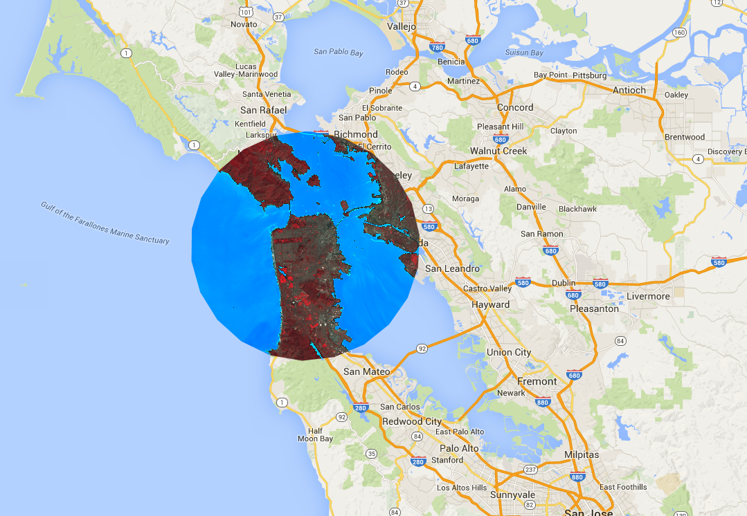
The paradigm.clip() method is useful for achieving cartographic furnishings. The following example clips the mosaic created previously to an arbitrary buffer zone around the metropolis of San Francisco:

Code Editor (JavaScript)

// Create a circle by drawing a 20000 meter buffer around a point. var roi = ee.Geometry.Point([-122.4481, 37.7599]).buffer(20000);  // Display a clipped version of the mosaic. Map.addLayer(mosaic.clip(roi), null, 'mosaic clipped');

Colab (Python)

# Create a circle by drawing a 20000 meter buffer effectually a point. roi = ee.Geometry.Point([-122.4481, 37.7599]).buffer(20000) mosaic_clipped = mosaic.prune(roi)  # Define a map centered on San Francisco. map_mosaic_clipped = folium.Map(location=[37.7599, -122.4481], zoom_start=10)  # Add the image layer to the map and display it. map_mosaic_clipped.add_ee_layer(mosaic_clipped, None, 'mosaic clipped') display(map_mosaic_clipped)

In the previous example, annotation that the coordinates are provided to the Geometry constructor and the buffer length is specified as 20,000 meters. Learn more than about geometries on the Geometries page.

The mosaic shown above, clipped to a buffer around San Francisco, California, United states of america.

Rendering categorical maps

Palettes are too useful for rendering discrete valued maps, for case a land cover map. In the instance of multiple classes, employ the palette to supply a dissimilar color for each grade. (The image.remap() method may be useful in this context, to convert arbitrary labels to consecutive integers). The following example uses a palette to render country cover categories:

Code Editor (JavaScript)

// Load 2012 MODIS land cover and select the IGBP classification. var cover = ee.Paradigm('MODIS/051/MCD12Q1/2012_01_01')   .select('Land_Cover_Type_1');  // Define a palette for the 18 distinct country cover classes. var igbpPalette = [   'aec3d4', // water   '152106', '225129', '369b47', '30eb5b', '387242', // wood   '6a2325', 'c3aa69', 'b76031', 'd9903d', '91af40',  // shrub, grass   '111149', // wetlands   'cdb33b', // croplands   'cc0013', // urban   '33280d', // crop mosaic   'd7cdcc', // snow and water ice   'f7e084', // barren   '6f6f6f'  // tundra ];  // Specify the min and max labels and the color palette matching the labels. Map.setCenter(-99.229, forty.413, v); Map.addLayer(encompass,              {min: 0, max: 17, palette: igbpPalette},              'IGBP classification');

Colab (Python)

# Load 2012 MODIS state encompass and select the IGBP classification. cover = ee.Paradigm('MODIS/051/MCD12Q1/2012_01_01').select('Land_Cover_Type_1')  # Define a palette for the 18 distinct land cover classes. igbp_palette = [     'aec3d4',  # water     '152106',     '225129',     '369b47',     '30eb5b',     '387242',  # forest     '6a2325',     'c3aa69',     'b76031',     'd9903d',     '91af40',  # shrub, grass     '111149',  # wetlands     'cdb33b',  # croplands     'cc0013',  # urban     '33280d',  # ingather mosaic     'd7cdcc',  # snow and ice     'f7e084',  # barren     '6f6f6f'   # tundra ]  # Define a map centered on the U.s.a.. map_palette = folium.Map(location=[xl.413, -99.229], zoom_start=5)  # Add the image layer to the map and display it. Specify the min and max labels # and the color palette matching the labels. map_palette.add_ee_layer(     cover, {'min': 0, 'max': 17, 'palette': igbp_palette}, 'IGBP classes') display(map_palette)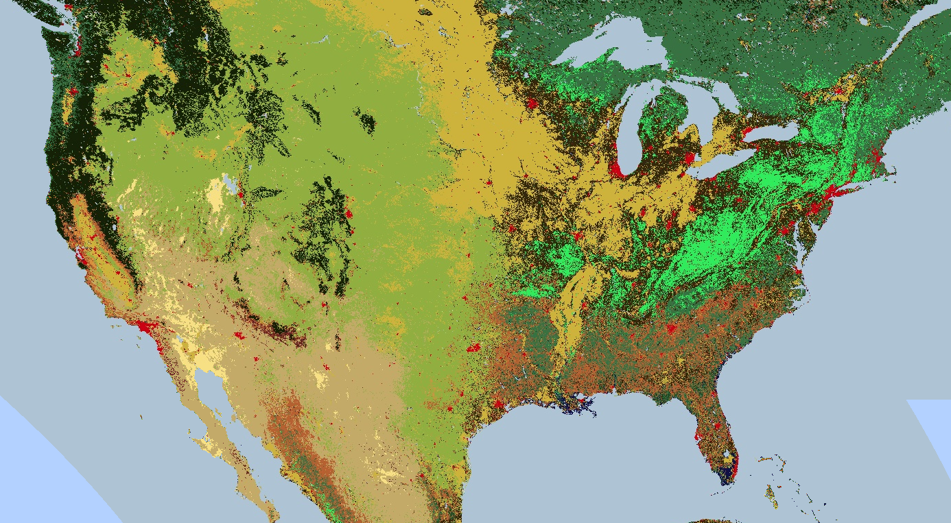

MODIS 2012 land cover using the IGBP nomenclature.

Styled Layer Descriptors

You can use a Styled Layer Descriptor (SLD) to render imagery for display. Provide epitome.sldStyle() with an XML description of the symbolization and coloring of the image, specifically the RasterSymbolizer chemical element. Acquire more well-nigh the RasterSymbolizer element hither. For example, to return the land cover map described in the Rendering categorical maps section with an SLD, apply:

Lawmaking Editor (JavaScript)

var cover = ee.Paradigm('MODIS/051/MCD12Q1/2012_01_01').select('Land_Cover_Type_1');  // Define an SLD fashion of detached intervals to apply to the image. var sld_intervals = '<RasterSymbolizer>' +   '<ColorMap type="intervals" extended="fake">' +     '<ColorMapEntry color="#aec3d4" quantity="0" label="H2o"/>' +     '<ColorMapEntry color="#152106" quantity="one" label="Evergreen Needleleaf Wood"/>' +     '<ColorMapEntry color="#225129" quantity="two" label="Evergreen Broadleaf Forest"/>' +     '<ColorMapEntry color="#369b47" quantity="3" characterization="Deciduous Needleleaf Forest"/>' +     '<ColorMapEntry color="#30eb5b" quantity="four" label="Deciduous Broadleaf Forest"/>' +     '<ColorMapEntry color="#387242" quantity="five" label="Mixed Deciduous Wood"/>' +     '<ColorMapEntry color="#6a2325" quantity="6" label="Closed Shrubland"/>' +     '<ColorMapEntry color="#c3aa69" quantity="7" label="Open up Shrubland"/>' +     '<ColorMapEntry colour="#b76031" quantity="8" characterization="Woody Savanna"/>' +     '<ColorMapEntry color="#d9903d" quantity="nine" label="Savanna"/>' +     '<ColorMapEntry color="#91af40" quantity="x" label="Grassland"/>' +     '<ColorMapEntry color="#111149" quantity="11" label="Permanent Wetland"/>' +     '<ColorMapEntry color="#cdb33b" quantity="12" label="Cropland"/>' +     '<ColorMapEntry colour="#cc0013" quantity="xiii" label="Urban"/>' +     '<ColorMapEntry color="#33280d" quantity="xiv" label="Ingather, Natural Veg. Mosaic"/>' +     '<ColorMapEntry color="#d7cdcc" quantity="15" label="Permanent Snow, Ice"/>' +     '<ColorMapEntry color="#f7e084" quantity="sixteen" label="Barren, Desert"/>' +     '<ColorMapEntry color="#6f6f6f" quantity="17" label="Tundra"/>' +   '</ColorMap>' + '</RasterSymbolizer>'; Map.addLayer(comprehend.sldStyle(sld_intervals), {}, 'IGBP classification styled');

Colab (Python)

embrace = ee.Image('MODIS/051/MCD12Q1/2012_01_01').select('Land_Cover_Type_1')  # Define an SLD style of detached intervals to utilise to the image. sld_intervals = """ <RasterSymbolizer>   <ColorMap  type="intervals" extended="false" >     <ColorMapEntry colour="#aec3d4" quantity="0" label="Water"/>     <ColorMapEntry color="#152106" quantity="1" label="Evergreen Needleleaf Forest"/>     <ColorMapEntry color="#225129" quantity="2" label="Evergreen Broadleaf Woods"/>     <ColorMapEntry color="#369b47" quantity="3" label="Deciduous Needleleaf Forest"/>     <ColorMapEntry color="#30eb5b" quantity="four" characterization="Deciduous Broadleaf Forest"/>     <ColorMapEntry colour="#387242" quantity="v" characterization="Mixed Deciduous Woods"/>     <ColorMapEntry color="#6a2325" quantity="vi" label="Closed Shrubland"/>     <ColorMapEntry color="#c3aa69" quantity="7" characterization="Open Shrubland"/>     <ColorMapEntry colour="#b76031" quantity="eight" characterization="Woody Savanna"/>     <ColorMapEntry color="#d9903d" quantity="9" label="Savanna"/>     <ColorMapEntry color="#91af40" quantity="10" label="Grassland"/>     <ColorMapEntry color="#111149" quantity="11" characterization="Permanent Wetland"/>     <ColorMapEntry color="#cdb33b" quantity="12" label="Cropland"/>     <ColorMapEntry color="#cc0013" quantity="xiii" label="Urban"/>     <ColorMapEntry color="#33280d" quantity="14" label="Crop, Natural Veg. Mosaic"/>     <ColorMapEntry color="#d7cdcc" quantity="15" label="Permanent Snow, Ice"/>     <ColorMapEntry colour="#f7e084" quantity="16" label="Barren, Desert"/>     <ColorMapEntry color="#6f6f6f" quantity="17" characterization="Tundra"/>   </ColorMap> </RasterSymbolizer>"""  # Apply the SLD fashion to the image. cover_sld = embrace.sldStyle(sld_intervals)  # Define a map centered on the United States. map_sld_categorical = folium.Map(location=[40.413, -99.229], zoom_start=5)  # Add the image layer to the map and display it. map_sld_categorical.add_ee_layer(cover_sld, None, 'IGBP classes styled') brandish(map_sld_categorical)

To create a visualization image with a color ramp, set the blazon of the ColorMap to 'ramp'. The following example compares the 'interval' and 'ramp' types for rendering a DEM:

Code Editor (JavaScript)

// Load SRTM Digital Elevation Model data. var image = ee.Paradigm('CGIAR/SRTM90_V4');  // Define an SLD way of detached intervals to apply to the image. var sld_intervals =   '<RasterSymbolizer>' +     '<ColorMap type="intervals" extended="false" >' +       '<ColorMapEntry color="#0000ff" quantity="0" label="0"/>' +       '<ColorMapEntry color="#00ff00" quantity="100" label="1-100" />' +       '<ColorMapEntry colour="#007f30" quantity="200" characterization="110-200" />' +       '<ColorMapEntry color="#30b855" quantity="300" label="210-300" />' +       '<ColorMapEntry color="#ff0000" quantity="400" label="310-400" />' +       '<ColorMapEntry colour="#ffff00" quantity="m" label="410-chiliad" />' +     '</ColorMap>' +   '</RasterSymbolizer>';  // Define an sld style color ramp to use to the paradigm. var sld_ramp =   '<RasterSymbolizer>' +     '<ColorMap type="ramp" extended="false" >' +       '<ColorMapEntry color="#0000ff" quantity="0" label="0"/>' +       '<ColorMapEntry color="#00ff00" quantity="100" label="100" />' +       '<ColorMapEntry color="#007f30" quantity="200" label="200" />' +       '<ColorMapEntry color="#30b855" quantity="300" characterization="300" />' +       '<ColorMapEntry color="#ff0000" quantity="400" label="400" />' +       '<ColorMapEntry color="#ffff00" quantity="500" characterization="500" />' +     '</ColorMap>' +   '</RasterSymbolizer>';  // Add the prototype to the map using both the color ramp and interval schemes. Map.setCenter(-76.8054, 42.0289, 8); Map.addLayer(paradigm.sldStyle(sld_intervals), {}, 'SLD intervals'); Map.addLayer(image.sldStyle(sld_ramp), {}, 'SLD ramp');

Colab (Python)

# Load SRTM Digital Tiptop Model data. image = ee.Image('CGIAR/SRTM90_V4')  # Define an SLD style of discrete intervals to utilise to the image. sld_intervals = """     <RasterSymbolizer>       <ColorMap type="intervals" extended="fake" >         <ColorMapEntry color="#0000ff" quantity="0" label="0"/>         <ColorMapEntry colour="#00ff00" quantity="100" label="one-100" />         <ColorMapEntry colour="#007f30" quantity="200" characterization="110-200" />         <ColorMapEntry color="#30b855" quantity="300" characterization="210-300" />         <ColorMapEntry color="#ff0000" quantity="400" label="310-400" />         <ColorMapEntry color="#ffff00" quantity="1000" label="410-grand" />       </ColorMap>     </RasterSymbolizer>"""  # Define an sld way color ramp to utilise to the paradigm. sld_ramp = """     <RasterSymbolizer>       <ColorMap type="ramp" extended="fake" >         <ColorMapEntry color="#0000ff" quantity="0" label="0"/>         <ColorMapEntry color="#00ff00" quantity="100" label="100" />         <ColorMapEntry color="#007f30" quantity="200" characterization="200" />         <ColorMapEntry color="#30b855" quantity="300" label="300" />         <ColorMapEntry color="#ff0000" quantity="400" label="400" />         <ColorMapEntry colour="#ffff00" quantity="500" characterization="500" />       </ColorMap>     </RasterSymbolizer>"""  # Ascertain a map centered on the United States. map_sld_interval = folium.Map(location=[40.413, -99.229], zoom_start=5)  # Add the image layers to the map and brandish information technology. map_sld_interval.add_ee_layer(     prototype.sldStyle(sld_intervals), None, 'SLD intervals') map_sld_interval.add_ee_layer(prototype.sldStyle(sld_ramp), None, 'SLD ramp') brandish(map_sld_interval.add_child(folium.LayerControl()))

SLDs are too useful for stretching pixel values to improve visualizations of continuous data. For instance, the following code compares the results of an capricious linear stretch with a min-max 'Normalization' and a 'Histogram' equalization:

Code Editor (JavaScript)

// Load a Landsat 8 raw image. var image = ee.Prototype('LANDSAT/LC08/C02/T1/LC08_044034_20140318');  // Define a RasterSymbolizer element with '_enhance_' for a placeholder. var template_sld =   '<RasterSymbolizer>' +     '<ContrastEnhancement><_enhance_/></ContrastEnhancement>' +     '<ChannelSelection>' +       '<RedChannel>' +         '<SourceChannelName>B5</SourceChannelName>' +       '</RedChannel>' +       '<GreenChannel>' +         '<SourceChannelName>B4</SourceChannelName>' +       '</GreenChannel>' +       '<BlueChannel>' +         '<SourceChannelName>B3</SourceChannelName>' +       '</BlueChannel>' +     '</ChannelSelection>' +   '</RasterSymbolizer>';  // Get SLDs with unlike enhancements. var equalize_sld = template_sld.supercede('_enhance_', 'Histogram'); var normalize_sld = template_sld.replace('_enhance_', 'Normalize');  // Display the results. Map.centerObject(epitome, 10); Map.addLayer(image, {bands: ['B5', 'B4', 'B3'], min: 0, max: 15000}, 'Linear'); Map.addLayer(image.sldStyle(equalize_sld), {}, 'Equalized'); Map.addLayer(image.sldStyle(normalize_sld), {}, 'Normalized');

Colab (Python)

# Load a Landsat 8 raw image. epitome = ee.Image('LANDSAT/LC08/C02/T1/LC08_044034_20140318')  # Define a RasterSymbolizer element with '_enhance_' for a placeholder. template_sld = """ <RasterSymbolizer>   <ContrastEnhancement><_enhance_/></ContrastEnhancement>   <ChannelSelection>     <RedChannel>       <SourceChannelName>B5</SourceChannelName>     </RedChannel>     <GreenChannel>       <SourceChannelName>B4</SourceChannelName>     </GreenChannel>     <BlueChannel>       <SourceChannelName>B3</SourceChannelName>     </BlueChannel>   </ChannelSelection> </RasterSymbolizer>"""  # Get SLDs with unlike enhancements. equalize_sld = template_sld.replace('_enhance_', 'Histogram') normalize_sld = template_sld.supersede('_enhance_', 'Normalize')  # Ascertain a map centered on San Francisco Bay. map_sld_continuous = folium.Map(location=[37.5010, -122.1899], zoom_start=x)  # Add the paradigm layers to the map and brandish it. map_sld_continuous.add_ee_layer(     epitome, {'bands': ['B5', 'B4', 'B3'], 'min': 0, 'max': 15000}, 'Linear') map_sld_continuous.add_ee_layer(     image.sldStyle(equalize_sld), None, 'Equalized') map_sld_continuous.add_ee_layer(     image.sldStyle(normalize_sld), None, 'Normalized') display(map_sld_continuous.add_child(folium.LayerControl()))

Points of note in reference to using SLDs in Earth Engine:

• OGC SLD ane.0 and OGC SE i.1 are supported.
• The XML document passed in can be consummate, or only the RasterSymbolizer element and downward.
• Bands may be selected by their Earth Engine names or index ('ane', '2', ...).
• The Histogram and Normalize contrast stretch mechanisms are non supported for floating point imagery.
• Opacity is only taken into account when information technology is 0.0 (transparent). Not-zero opacity values are treated as completely opaque.
• The OverlapBehavior definition is currently ignored.
• The ShadedRelief mechanism is not currently supported.
• The ImageOutline mechanism is non currently supported.
• The Geometry chemical element is ignored.
• The output paradigm volition have histogram_bandname metadata if histogram equalization or normalization is requested.

Thumbnail images

Use the ee.Paradigm.getThumbURL() method to generate a PNG or JPEG thumbnail image for an ee.Image object. Printing the consequence of an expression ending with a telephone call to getThumbURL() results in a URL being printed. Visiting the URL sets World Engine servers to work on generating the requested thumbnail on-the-fly. The epitome is displayed in a browser when processing completes. Information technology tin can be downloaded past selecting appropriate options from the image'due south correct-click context carte du jour.

SRTM digital elevation model displayed every bit a PNG thumbnail in a browser.

The getThumbURL() method includes parameters, described in the visualization parameters table in a higher place. Additionally, it takes optional dimensions, region, and crs arguments that control the spatial extent, size, and display project of the thumbnail.

Additional parameters for ee.Image.getThumbURL() with annotation on format

Parameter	Clarification	Type
dimensions	Thumbnail dimensions in pixel units. If a unmarried integer is provided, it defines the size of the epitome'due south larger aspect dimension and scales the smaller dimension proportionally. Defaults to 512 pixels for the larger image aspect dimension.	A single integer or string in the format: 'WIDTHxHEIGHT'
region	The geospatial region of the image to return. The whole image by default, or the bounds of a provided geometry.	GeoJSON or a 2-D list of at least three point coordinates that define a linear band
crs	The target project e.thou. 'EPSG:3857'. Defaults to WGS84 ('EPSG:4326').	String
format	Defines thumbnail format every bit either PNG or JPEG. The default PNG format is implemented as RGBA, where the alpha channel represents valid and invalid pixels, defined by the prototype's mask(). Invalid pixels are transparent. The optional JPEG format is implemented as RGB, where invalid image pixels are cipher filled beyond RGB channels.	Cord; either 'png' or 'jpg'

A single-band prototype will default to grayscale unless a palette argument is supplied. A multi-band image will default to RGB visualization of the first three bands, unless a bands argument is supplied. If merely two bands are provided, the first band will map to red, the 2nd to blueish, and the green channel volition exist zero filled.

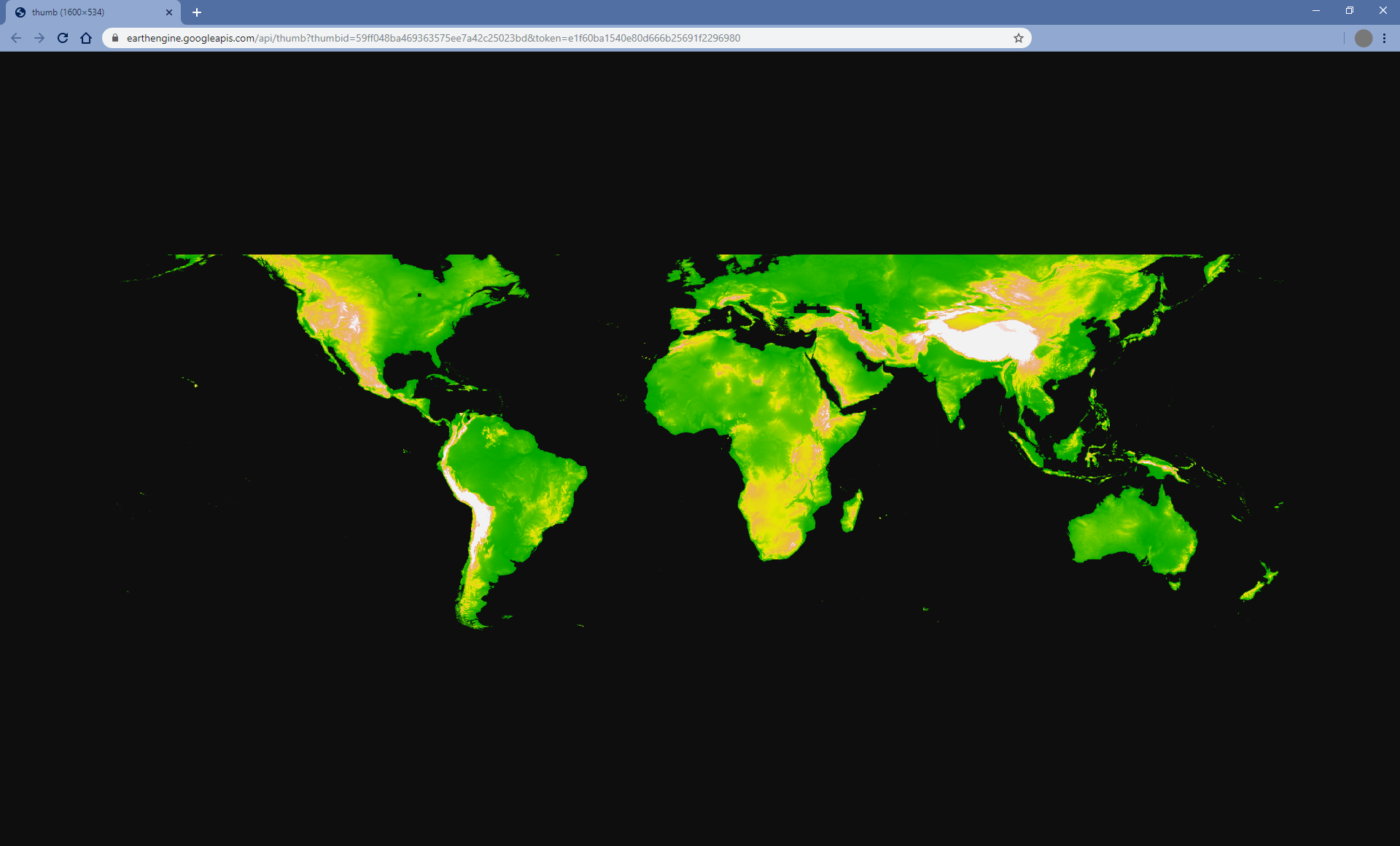
The post-obit are a series of examples demonstrating various combinations of getThumbURL() parameter arguments. Click on the URLs printed when you run this script to view the thumbnails.

Lawmaking Editor (JavaScript)

// Fetch a digital elevation model. var epitome = ee.Image('CGIAR/SRTM90_V4');  // Asking a default thumbnail of the DEM with defined linear stretch. // Set masked pixels (ocean) to 1000 and so they map as gray. var thumbnail1 = image.unmask(1000).getThumbURL({   'min': 0,   'max': 3000,   'dimensions': 500, }); print('Default extent:', thumbnail1);  // Specify region by rectangle, ascertain palette, ready larger aspect dimension size. var thumbnail2 = image.getThumbURL({   'min': 0,   'max': 3000,   'palette': ['00A600','63C600','E6E600','E9BD3A','ECB176','EFC2B3','F2F2F2'],   'dimensions': 500,   'region': ee.Geometry.Rectangle([-84.6, -55.9, -32.9, xv.7]), }); impress('Rectangle region and palette:', thumbnail2);  // Specify region by a linear ring and set brandish CRS as Web Mercator. var thumbnail3 = image.getThumbURL({   'min': 0,   'max': 3000,   'palette': ['00A600','63C600','E6E600','E9BD3A','ECB176','EFC2B3','F2F2F2'],   'region': ee.Geometry.LinearRing([[-84.6, fifteen.7], [-84.6, -55.9], [-32.nine, -55.ix]]),   'dimensions': 500,   'crs': 'EPSG:3857' }); print('Linear ring region and specified crs', thumbnail3);

Colab (Python)

# Fetch a digital peak model. image = ee.Prototype('CGIAR/SRTM90_V4')  # Request a default thumbnail of the DEM with defined linear stretch. # Set up masked pixels (ocean) to g so they map equally gray. thumbnail_1 = image.unmask(1000).getThumbURL({     'min': 0,     'max': 3000,     'dimensions': 500, }) impress('Default extent:', thumbnail_1)  # Specify region past rectangle, define palette, set larger aspect dimension size. thumbnail_2 = image.getThumbURL({     'min': 0,     'max': 3000,     'palette': [         '00A600', '63C600', 'E6E600', 'E9BD3A', 'ECB176', 'EFC2B3', 'F2F2F2'     ],     'dimensions': 500,     'region': ee.Geometry.Rectangle([-84.six, -55.ix, -32.nine, fifteen.7]), }) impress('Rectangle region and palette:', thumbnail_2)  # Specify region by a linear band and gear up display CRS as Web Mercator. thumbnail_3 = image.getThumbURL({     'min': 0,     'max': 3000,     'palette': [         '00A600', '63C600', 'E6E600', 'E9BD3A', 'ECB176', 'EFC2B3', 'F2F2F2'     ],     'region':         ee.Geometry.LinearRing([[-84.half-dozen, fifteen.7], [-84.six, -55.ix], [-32.9, -55.nine]]),     'dimensions': 500,     'crs': 'EPSG:3857' }) print('Linear ring region and specified crs:', thumbnail_3)

Except as otherwise noted, the content of this page is licensed under the Creative Eatables Attribution 4.0 License, and code samples are licensed under the Apache 2.0 License. For details, see the Google Developers Site Policies. Coffee is a registered trademark of Oracle and/or its affiliates.

Last updated 2021-05-27 UTC.

campchereappleas.blogspot.com

Source: https://developers.google.com/earth-engine/guides/image_visualization